00:00
Hello, everyone, and thanks for listening to a talk, entitled "Reinforcement Learning Integrated with Supervised Learning for Training of Near Infrared Spectrum Data for Non-destructive Testing of Fruits." My name is Simarjeet Saini. And the co-authors are Yuqi Li and Kulbir Ahluwalia. This work was done at the University of Waterloo in Canada.
00:33
We'll begin the presentation with a quick introduction towards the use of MI spectroscopy for non-destructive food quality measurements and why we felt there was a need for machine learning models which could auto-train the data. The data collection for the study will be described, followed by model description for auto-training. Finally, we'll describe the results and conclude the presentation.
01:03
Over the last few decades, visible and near-infrared spectroscopy has shown promise for non-destructive quality measurements. And IR systems today are being widely used in packing lines. Fruits and vegetables have chemical groups with oxygen-hydrogen, carbon-hydrogen, and nitrogen-hydrogen bonds which have absorption peaks in the visible near-infrared spectrum. Various training algorithms have been used to convert the absorption spectra to meaningful metrics describing the quality parameters-- for example, the solid soluble content, [INAUDIBLE] matter, vitamin concentration, et cetera.
01:50
The various models which have been used over the last few years, the models normally have three different stages-- the input data set, pre-processing methods, and the discriminant methods. The reflectance data is normally converted to absorbance data and the first and second order derivatives taken.
02:21
The data is then properly processed with methods like moving average smoothing, detrending standard normal variate, principal component analysis, et cetera. In our experience, the pre-processing steps play a very important role in the ultimate accuracy of the trained models. Different discriminant methods-- like support vector machine, partial least square regression, decision tree, and artificial neural networks-- have been demonstrated for building the prediction models and getting the meaningful quality metrics.
03:04
With a plethora of choices available, it is not always clear which combination provides the globalized optimal results for the given data set. Going through various combinations is very time-consuming. And the optimization depends upon the experience of the analyst. So [AUDIO OUT] arose for us, which was whether it would be possible to use machine learning methods to choose and optimize the best combination of these algorithms automatically without any user interface intervention.
03:49
This presentation describes some of our work in developing such a model. To build and test the model, experiments were done to predict the solid soluble content for kiwi fruit 378 samples were procured from two different retail chains, directly from the distribution centers.
04:22
The SSC values ranged from 7.3% to 6.1% for the samples. Approximately 30 kiwi fruits were measured every day over 12 consecutive days. They were stored in a refrigerator at 5 degrees C and relative humidity of approximately 80% when not undergoing measurement. Before measurements, the kiwifruit were taken out of the refrigerator and placed in the ambient surrounding for one hour to reach room temperature.
04:55
The temperature of the room was maintained at 22 degrees C with a relative humidity of approximately 40% throughout the experimentation process. Of the 378 fruits, 266 were used to train the calibration models. And 112 were used to test the models for the values of SSC. The detailed statistics of the population distribution are shown in the table here, and you can pause the video if you would like to see the details.
05:30
Spectroscopy was done with diffused reflectants using a [INAUDIBLE] setup consisting of Ocean Optics Jazz Spectrometer, with wavelength lengths spanning from 400 nanometers to 1,100 nanometers, and a spectral resolution of approximately 2 nanometers. Light from Ocean Optics halogen lamp with emission from 317 nanometers to 2,400 nanometers was coupled into an optical fiber with 1-millimeter core diameter.
06:12
The reflected light was collected with a 50 micron core optical fiber. A home built fiber holder was created in an aluminum block, such that the incident fiber was at a 45-degree angle to the sample, and the collection fiber was normal to the sample. The centers of the two fibers were displaced by approximately 8 millimeters.
06:40
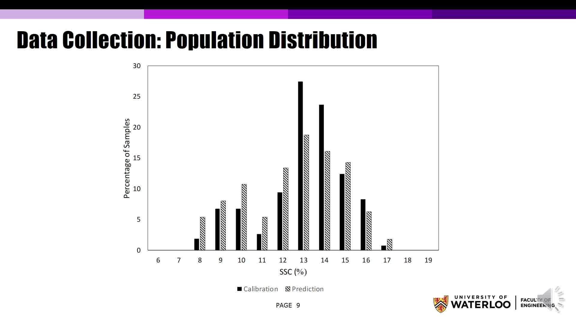
The sample holder was placed gently on the fruit to collect the reflection spectrum. The reflection spectrum was measured at three different points on the equator. Five different measurements were done at each point and the spectra averaged. Further, the scans were averaged over the three points. After the non-destructive measurements, Kiwis were cut in half, and SSC values measured with a Brix meter, three times for each half.
07:20
And the values were averaged to get the SSC value for the fruit. The figure plots the distribution of SSC for calibration and the prediction data set, respectively. For SSC, the distribution was bimodal, with major distribution around average value, while another weaker distribution was observed at around 10%.
07:53
The distributions were nearly similar for the calibration and the prediction data set, with the exception of a large number of lower SSC kiwi fruit than the prediction data set. The two data sets were randomly generated with a probability of 33% to be selected as a prediction-- to be selected as a prediction data point.
08:25
The photo on the slide shows the overall process to build a machine learning model. The model construction begins as a black box with the input data matrix, pre-processing methods, and discriminant methods chosen as the inputs. As for the output of the model, the model selects the best performed combination of one discriminant method, one compound of input categories and one compound of pre-processing methods, along with the optimize parameters within the algorithm.
09:06
In detail, the model conducts a grid search on the algorithm combinations, with a reinforcement loop as part of the grid search. The optimization process on each combination is visualized in terms of model map and model agents. Based on this visualization, reinforcement learning is applied on the agents. As the result, the location of the most outstanding agent represents the output of the model and the optimization.
09:45
To understand how the model works we need to understand these various components. But you can pause the video here to look at the various elements in detail. If you re-look at the various components. We should describe the two key assumptions we make. First one is, whether in function combination or not, key parameters will not change to non-key parameters.
10:16
The function combination can either be a combination of pre-processing methods or the combination between a discriminant method and the pre-processing method. This assumption provides a condition under which the model is able to identify the key parameters on each algorithm one by one. Without this assumption, the model has to identify new key parameters whenever new function combinations are created, which comes at a very high computing price.
10:52
Avoiding the high price to identify key parameters, this assumption dramatically increases the efficiency of the training process. But it might also potentially reduce the model accuracy. The second assumption is the number of pre-processing algorithms in combination should be less than or equal to sum n. And in this case, we have used n is equal to 4. What we were concerned is, that if we allow three number of combinations, then the data set might get over-preprocessed.
11:33
This assumption allows the model to avoid feature loss and save on training costs. Even though the largest size of pre-processing method combinations can be customized, we have kept it less than n is equal to 4. And as we will see in the results, we achieved the best results with a combination of two. To understand how the model works, we created a model map envisioned as a hill, which is the interaction result between factors and the portions of the algorithm.
12:19
Every algorithm combination corresponds to one model map. The dimensions of the map are the key parameters selected from the methods in the algorithm combination. Those key parameters change the factors and portions, thereby impacting the accuracy of the model. The accuracy is represented as height in this map. However, the height at the same location does not stay in the same value all the time.
12:53
Due to the randomicity from most discriminant methods, the height would keep changing in the specific range, which is called model variation. In the project, the range is regulated by a confidence interval whose default value of confidence level is 95%. Within this model, model agents are created to find the highest location in the model map.
13:25
These agents are originally spread throughout the map randomly. And their movements depend upon the mode they are set in, creating processes split into end periods on a box. In each period, climbers are able to move more than one step for an iteration. After one epoch, only a set number of top-performing agents are kept in the next start.
13:57
New agents are then created near the surviving agents before the new epoch would start. This reproduction process creates the reinforcement learning within our supervised learning model. The agents have three different modes of motion-- 360-degree detection, random detection, and random movement. And these modes are assigned to the agent at the start of an epoch.
14:32
Under the mode 360-degree detection, the detector attempts to step in both directions where the key parameter value is either increased or decreased before the agent decides to move. The mode 360-degree detection encourages the agent to scan slope values on each possible direction and then move towards the steepest slope, and thus should give the most optimal results.
15:17
However, this is computationally expensive. So only a small number of the agents are turned on in this mode. When a random detection move is chosen, the agent first repeats the same movement at the last step-- as in the first step. If the agent did not make a progress that is larger than the model variations trend, then it would randomly activate one of the detectors.
15:52
Once one of the detectors found slopes where climbers are able to improve the value that is larger than model variations trend, the climbers would stop activating, and the remaining detectors in the model would start to move-- or the agent would start to move in that direction. In a random movement, agents randomly choose a direction of movement without any care of whether it is climbing up the hill or falling down the hill.
16:24
An adaptive training learning rate was used for training the agents. The more progress an agent made at the last step, the less the learning rate would be applied on this agent. This configuration allows the agents to be more cautious when they're locating a hill or a cliff. Connected to the agents, the detectors of the agents, are tuners.
16:58
After collecting geometric information about the map, detectors return a tuning code to the tuners. The tuning code tells the climber to increase or decrease or keep still in dimension. By applying learning rate, tuners ask the agent to move to a new location and return the new values of key parameters. The reinforcement loop follows the rule of survival of the fittest at the end of the epoch.
17:31
The larger the progress the agent makes, the larger its likelihood of survival. The number of agents that are created and killed at different times are different for agents set in different modes. It is obvious that the climbers in the mode 360-degree detection cost the most computationally before movements. But the climbers in random movement do not cost computationally at all.
18:03
So the probability of survival for 360-degree detection is kept higher than the probability of survival for the random movement. While this model was working and always climbing up the hill, the major issue we faced was the computationally intensive nature of the full grid search used in the previous model. And thus, we could not really optimize the parameters.
18:37
Thus, in the next step, what we did was we broke the model training into two steps. In the first step, we optimized only for pre-processing combination by using partial least square regression as the discriminant method. In step 2, we assumed that the pre-processing combination will work well for all discriminant models and then used a novel integrated Deep Q learning method to optimize the discriminant model.
19:11
For the pre-processing algorithm combination, model agents only used random detection mode. Then groups were created with 4 individual agents in each group. And the model was run for 20 epochs. Each group of agents had a random compilation of pre-processing methods assigned to it, and the individuals in the group had different rates.
19:45
There were four iterations of steps within each epoch. After each epoch, two agents in each group survived, and four new agents were randomly created around each of the surviving ones. After 20 epochs, what we found was that the absorption spectra, without first and second [INAUDIBLE],, just the absorption spectra, treated with multiplicative scatter correction and standard normal variate correction gave the highest accuracy.
20:20
And thus, the data was pre-processed with these two algorithms. [AUDIO OUT] next step, we developed a new method for discriminative optimization. At the current time, we have only optimized one discrimination model to see whether this method works.
20:44
The optimization technique uses a primary model whose parameter we need to optimize and a secondary model which is used to optimize the parameters of the primary model. This methodology creates multiple modeling configurations and selects the one with the highest accuracy. By minimizing the number of trials, it saves a significant amount of computing power and computing time.
21:17
But there is a trade-off, and the trade-off is instead of searching for the configuration having the global maximum accuracy, the secondary reinforcement learning model automatically used the combination of the primary model and returns the best configuration that correlates to a local maximum accuracy of the primary model. For the present work, our primary model was support vector machine as the discriminant model for the prediction of SSC.
21:53
SVM is a regression model classifying all prediction lines to pass through a boundary or not. It uses a kernel to map dimensions to higher or lower dimensions. We used agents to optimize the kernel coefficient gamma and the regularization coefficient C. The secondary model used Deep Q learning. And this was used to train the parameters for the support vector machine.
22:26
DQN is a type of model-free reinforcement learning. But a play mechanism allows the model to apply Q learning on a [INAUDIBLE] basis. The introduced discount factor prioritized earlier reward over later ones. For the current work, we have used two-layer, fully connected MLP neural network in the DQN with 200 neurons in each layer.
23:00
To create a reinforcement learning policy, a state is created which consists of detection, gradient momentum, and configuration, as shown by the equations here. Each agent plays a game with different steps. Each game consists of a random walk within the SVM parameters, followed by an optimization with the Deep Q network.
23:34
The parameters from the random walk are fed into DQN optimization, where Q learning model is applied to further tune the parameters of the agent. Multiple agents are created to span an exhaustive search. An action increases or decreases the value [INAUDIBLE] by a predefined amount. And in a step, the action is applied and the state changed.
24:10
Reward is calculated and stored. There are two ways we end the game. One is when the agent runs out of the step limit as defined by the user. Otherwise, a game is terminated when the agent stays idle in a few recent steps. The idle state is triggered when the rewards in a predefined number of steps fail to show a minimum change over a threshold.
24:39
The idle state is essential to avoid adding bias and meaningless movement into the agent's memory. The results shown here show how the model optimizes with respect to one specific parameter within the model. Blue line is the full grid optimization of the results with respect to the parameter.
25:13
The y-axis blots the accuracy of prediction measured by the R-squared values. Marker in yellow here represents the highest accuracy achieved with a full grid search. At the start of game 1, 10 agents were randomly distributed and shown in this map with red. Some of the agents lie on top of each other as they get nearly similar accuracies.
25:47
After the end of game 1, the 10 agents performed quite differently. Some of them moved up the hill, closer to the optimal value, whereas others, not so much. The agents closer to the mountaintop were more adapted to this map geometry. At the beginning of game 2, one of the agents with the highest accuracy was chosen.
26:18
And then 10 agents were created to locations randomly chosen around one of the best performing agents from the previous game. At the end of the game 2, the 10 agents re-stepped away from the new starting point-- some moving closer to the optimal value and others falling off the hill. If we consider the highest performing agent, then its accuracy is only 1% lower than the highest accuracy achieved by the full grid search.
26:57
Within two games, R-squared value of 87% is achieved, with a root mean square error or 0.65%. It only took approximately 1% to 2% of the time to come closer to the peak accuracy as compared to a full grid search, thus removing the issue we had faced before. In the future, this method of optimization will allow us to implement the complete model for building train models automatically through machine learning.
27:35
Based on the SVM optimization with the previous method, we achieved an R-squared of 0.92 and a root mean square error for prediction of 0.65% for the given data set. The results are actually better than other studies using the same wavelength range for prediction of SSC for kiwis, as was discussed in another paper in the same conference.
28:04
So in conclusion, we have proposed a model combining reinforced learning with supervised learning and demonstrated its use and optimization of combination of pre-treatment methods. We have presented how reinforcement learning can be used to model configuration tasks. We are excited about the potential of the optimization methodology on other primary models, such as neural networks.
28:37
And at this point, I would love to have your questions and suggestions for improving our work. Thanks a lot.


